6. Examples

In the following sections we present some simplified examples and use Aronnax to reproduce a number of published results to show how Aronnax can be easily configured for a range of idealised modelling studies.

6.1. Canonical examples

These simulations use simple domains and and inputs. They highlight some of the features available in Aronnax and can be found in the examples/ folder. To run these simulations locally change into the examples/ directory and execute python run_examples.py in the terminal.

6.1.1. Gaussian bump on a \(\beta\)-plane

This example is initialised with a Gaussian bump in the layer thickness field. The momentum forcing is set to zero. The initial thickness of the upper layer for both examples is shown in Figure 6.1.

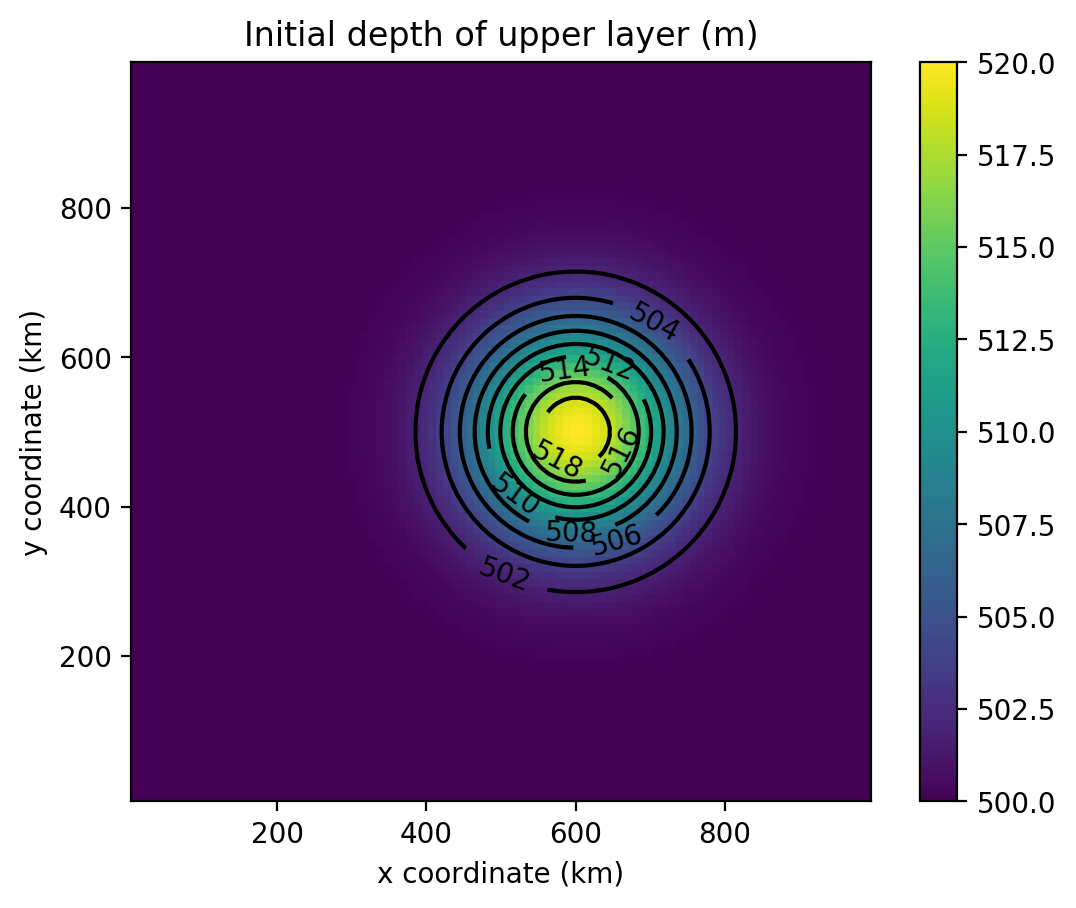
Figure 6.1 Initial thickness of the upper layer for the Gaussian bump examples

1 + 1/2 layers

Figure 6.2 Evolution of a Gaussian bump on a 1.5 layer \(\beta\)-plane.

2 layers

The upper layer of a two-layer simulation with a flat bottom. This looks very similar to the 1.5 layer simulation.

Figure 6.3 Evolution of a Gaussian bump on a 2 layer \(\beta\)-plane.

6.1.2. Twin gyre on a \(\beta\)-plane

These two examples begin with closed rectangular domains that are initially at rest. The momentum forcing shown in Figure 6.4 is applied to the upper layer in both examples. Due to it’s computational complexity the \(n\) layer configuration takes substantially longer to run than the \(n+1/2\) layer simulation.

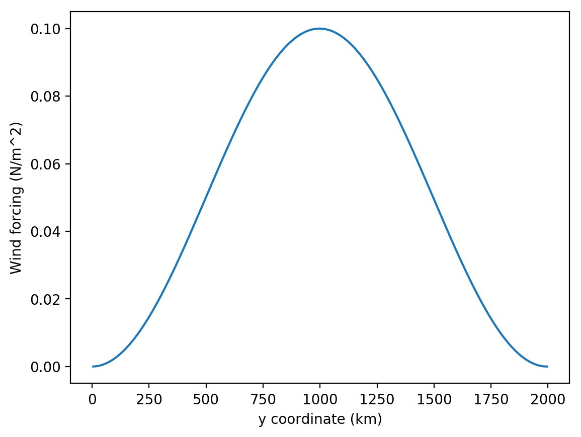
Figure 6.4 Zonal wind forcing applied to twin gyre simulations.

The twin gyre simulations are run on a 10 km resolution \(\beta\)-plane with Coriolis parameters equivalent to the midlatitudes of the Northern Hemisphere. At these latitudes 10 km is an eddy resolving resolution, and we expect to see inertial recirculations and internal variability develop as the simulations spin up.

1 + 1/2 layers

This example simulates a twin-gyre on a \(\beta\)-plane with 1 active layer above a quiescent abyss. This simulation runs for almost 140 days of model time, and clearly shows the development of the two gyres and inertial recirculations at the inter-gyre boundary.

Figure 6.5 Evolution of a twin-gyre on a 1.5 layer \(\beta\)-plane.

2 layers

This is also a twin-gyre simulation, but is run with \(n\) layer physics and a flat bottom. Once again the simulation runs for almost 140 model days and clearly shows the development of two gyres, western boundary currents, and inertial recirculation regions.

Figure 6.6 Evolution of a twin-gyre on a 2 layer \(\beta\)-plane.

6.2. Reproducing published results

These examples show how Aronnax can be used to reproduce results from the literature.

6.2.1. Davis et al. (2014) - An idealised Beaufort Gyre

Davis et al. (2014) used a reduced gravity model to explore the response of an idealised Beaufort Gyre to changes in the seasonal cycle of wind stress. Here we reproduce their control simulation. The domain is set up as a lollipop, with a circular basin for the Beaufort Gyre and a narrow channel connecting it to a region with sponges.

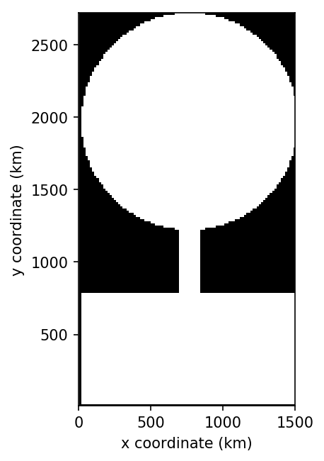
Figure 6.7 The computational domain for Davis et al. (2014). Note: the domain is symmetric, it is the plotting command that makes it look asymmetric.

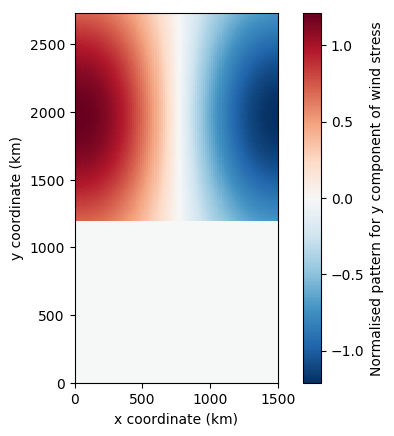
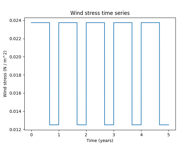
Over this lollipop basin a wind stress is used to drive an anticyclonic circulation. The magnitude of the wind stress is given as

(6.1)\[\frac{1}{r}\int{r \cos^{2}(r)} dr\]

which is multiplied by \(\sin(\theta)\) or \(-\cos(\theta)\) to give the x and y components of the wind stress. Converting the integral into the wind stress requires evaluating \(1/r\) times the integral as

(6.2)\[\frac{1}{r} \left(\frac{r \sin(2r)}{4} - \frac{\sin^{2}(r)}{4} + \frac{r^{2}}{4}\right)\]

and normalising the result such that the average wind stress magnitude inside the circular domain is equal to one. This normalised wind stress is then converted into its x and y components.

The y component of the normalised wind stress field is shown on the left, and the time series of wind stress magnitude is on the right.

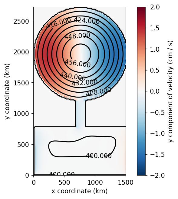
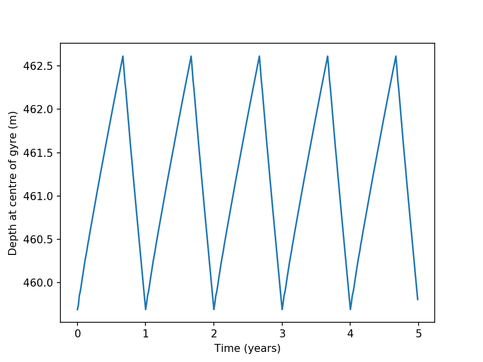
After integrating for 40 model years these inputs produce a steady seasonal cycle in velocity and layer thickness. A snap shot is shown on the left, while a time series of the maximum thickness is shown on the right.

The seasonal cycle in layer thickness requires a time varying transport through the channel. This is shown below.

Figure 6.8 Time series of transport through the channel due to the seasonal cycle in wind stress.

The paper includes multiple experiments perturbing the seasonal cycle of wind stress. Reproducing the perturbation experiments would require modifying the input variable wind_mag_time_series_file.

Note

The configuration used to create these outputs can be found in the reproductions folder of the repository.

6.2.2. Yang et al. (2016)

Yang et al. (2016) run and analyse a series of idealised n-layer models of the Beaufort Gyre in the Arctic. A configuration of Aronnax that mimics their setup can be found in the reproductions folder.

The spin up of the model proceeds as expected, but baroclinic instability sets in sooner than observed in the simulations by Yang et al. (2016). For this reason, the deepening of the upper layer is halted earlier, and it does not become as thick as in their simulations. There are multiple numerical differences between the model described by Yang et al. and Aronnax. For example, they use biharmonic viscosity and a quadratic bottom drag, while Aronnax has Laplacian viscosity and linear bottom drag. Numerical details can make a substantial difference to the output of numerical simulations, and these differences may be why Aronnax fails to reproduce the mean state of their model. The model state after 14 years of simulation is shown in Figure 6.9. Comparing Figure 6.9 with their Figure 3 highlights that the upper layer in the Aronnax simulation is thinner.

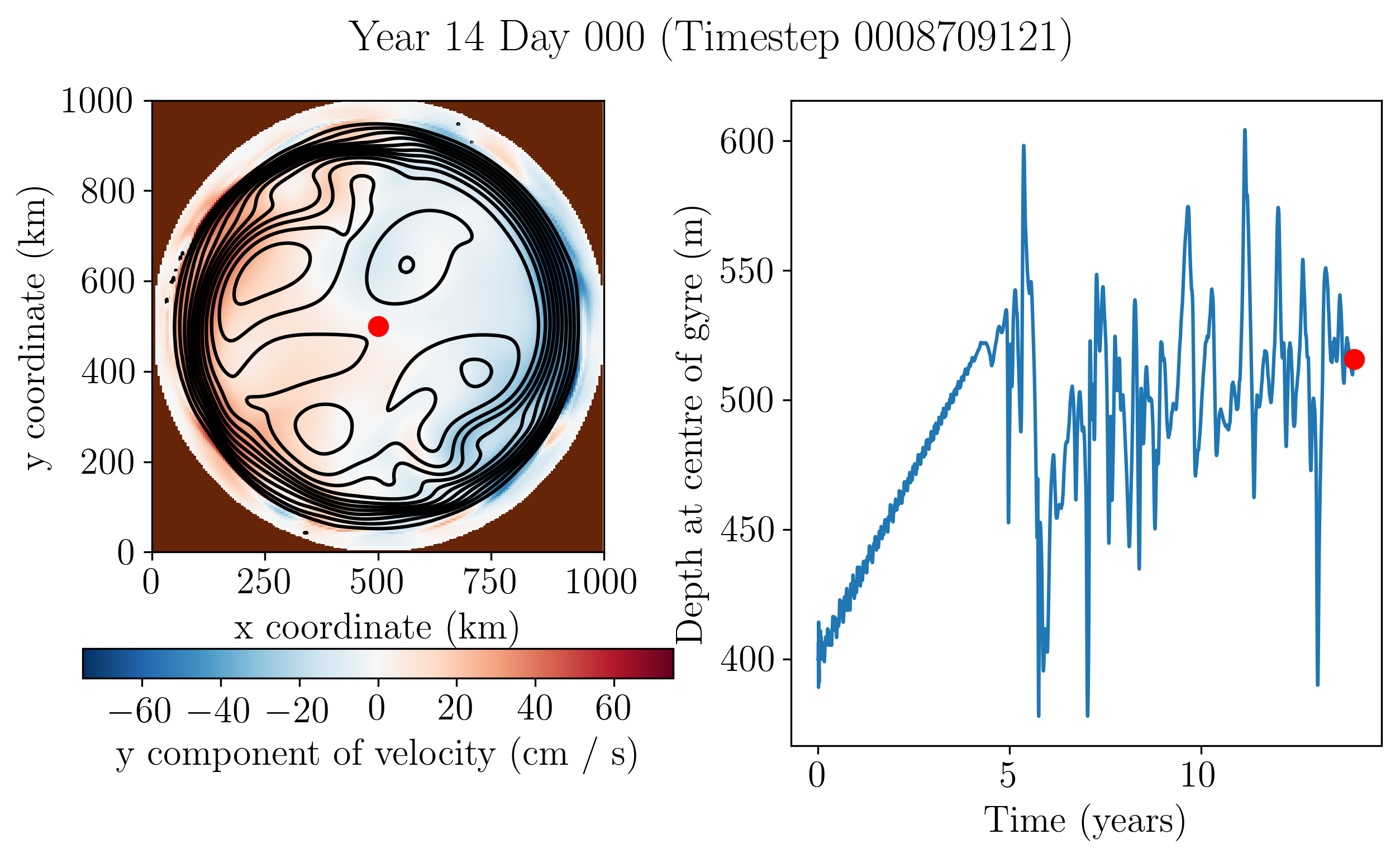
Figure 6.9 Left: Upper layer y velocity (colours) and thickness (contours). Right: Time series of thickness at centre of gyre.

An animation of the simulation can be seen below.

An interactive plot of the model state after 14 years of model time can be found below. The blue/grey surface shows a cutaway of the bathymetry.

Note

The configuration used to run this simulation can be found in the reproductions/Yang_et_al_2016 folder.

6.2.3. Manucharyan and Spall (2016)

n-layer configuration looking at eddies in the Arctic. (The original experiment was run using a z-level model, but it could also be done in an isopycnal model)

6.2.4. Johnson and Marshall (2002)

Reduced gravity analysis of the adjustment of the MOC to changes in deep water formation rates.